What Is a RAG Pipeline? Retrieval-Augmented Generation Works
A RAG pipeline retrieves relevant chunks from an external knowledge base and inserts them into an LLM’s prompt before it generates an answer. It fixes two core LLM problems — stale training data and hallucination — without retraining the model.
Prerequisites / Related Deep Dives: This guide assumes basic familiarity with LLM prompting. For background on specific building blocks referenced throughout, see: Vector Embeddings, Cross-Encoders & Rerankers, Knowledge Graphs & Graph Databases, and Prompt Caching.
A RAG pipeline (Retrieval-Augmented Generation pipeline) is a system that retrieves relevant information from an external knowledge source and feeds it to a large language model as context before the model generates a response. Instead of relying only on what it learned during training, the model answers using fresh, specific data pulled in at the moment of the query. The technique traces back to Lewis et al.’s 2020 paper introducing retrieval-augmented generation for knowledge-intensive NLP tasks, which set out the retrieve-then-generate approach that nearly all modern RAG systems still build on.
Core idea to remember: retrieve first, then generate. The “R” finds the facts; the “G” writes the answer.
The Structural Limit of Standalone LLMs (And Why Prompting Isn’t Enough)
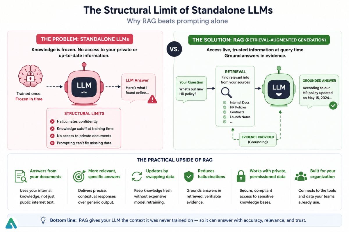
Standalone LLMs have two structural problems: they can hallucinate (state things confidently that aren’t true), and their knowledge is frozen at whenever training ended. They also can’t access your product launch from last week, your internal HR policy, or a contract your legal team just uploaded. You have two options — retrain the model (expensive, slow, and outdated again in a month) or give it access to a live source of truth at query time. RAG is the second option.
The practical upside:
Answers questions from your own documents, not just public internet text
Produces more relevant, specific answers instead of generic ones
Updates by swapping out data — no model retraining required
Reduces hallucinations by grounding answers in retrieved evidence
Works with private, permissioned knowledge bases
The Two Phases of a RAG Pipeline
Phase 1 — Offline Indexing (happens once, then periodically): The pipeline collects your documents, cleans them, splits them into chunks, converts them into embeddings, and stores them in a vector database. This is the prep work that makes real-time retrieval fast later on.
Phase 2 — Real-Time Retrieval (happens on every user query): A user asks a question. The system searches the vector database for the most relevant chunks and adds them to the prompt. The LLM then generates an answer using that context.
Collect documents — PDFs, wikis, support tickets, product manuals, whatever your knowledge base includes.
Clean the data — strip formatting noise, fix broken text extraction, remove duplicates.
Split documents into chunks — break large documents into smaller, manageable pieces.
Generate embeddings — convert each chunk into a numerical vector representing its meaning.
Store embeddings in a vector database — Pinecone, Weaviate, Milvus, Qdrant, or Chroma are common choices.
Receive the user query — the pipeline kicks into its real-time phase.
Retrieve relevant chunks — the pipeline embeds the query, then matches it against stored vectors by similarity.
Rerank results — a secondary model scores retrieved chunks for actual relevance, trimming noise.
Add context to the prompt — the pipeline inserts the top chunks alongside the user’s question.
Generate the answer — the LLM produces a response grounded in that retrieved context.
Provide citations — the best systems show which source chunks the answer came from, so it’s verifiable.
Key Components of a Production RAG Pipeline
Source Connectors & Ingestion
Real-world knowledge bases are messy — multi-column PDFs, scanned images needing OCR, tables, HTML pages with junk metadata. A production-grade pipeline needs solid extraction before anything else happens, because a bad ingestion step poisons every step after it.
Keeping the index in sync: the offline-indexing framing above implies a one-time job, but in production the source documents keep changing — a wiki page gets edited, a policy PDF gets replaced, a ticket gets closed. Two common approaches:
Scheduled batch re-indexing — re-embed the whole knowledge base (or changed files) on a cron schedule. Simple, but stale between runs.
Change Data Capture (CDC) — listen for change events at the source (database triggers, file-system watchers, webhook events from a CMS) and re-embed just the changed documents as they change. Lower staleness, more moving parts to maintain.
Which one makes sense depends on how often the underlying content actually changes — a static compliance archive doesn’t need CDC; a live product catalog usually does.
Chunking Strategies
Chunking splits documents into smaller pieces before embedding. Teams often underestimate this step, but chunking strategy has an outsized effect on retrieval quality — get it wrong, and even a well-tuned retriever pulls back the wrong information.
Common approaches:
Fixed-size chunking — split every N tokens, sometimes with overlap so context isn’t cut mid-sentence
Sentence or paragraph-based chunking — respects natural language boundaries
Semantic chunking — groups sentences by meaning rather than arbitrary length
Contextual chunk headers — injects the document title or summary into each chunk so it doesn’t lose context once separated from the original document
A common failure mode: naive fixed-size chunking can cut a sentence, table row, or code block in half at the boundary, which confuses both the reranker and the LLM. This is why sentence-aware, recursive, and semantic strategies exist.
Field note: this shows up hardest on financial and legal PDFs, where a single table can span a page and a fixed-size splitter has no concept of “don’t cut here.” Teams running large batches of scanned financial documents often see chunking-related retrieval failures concentrated almost entirely in tables and multi-column layouts — switching to a layout-aware or recursive splitter that respects table boundaries is usually the fix, not a bigger chunk size.
Where contextual chunk headers come from: this technique closely follows Anthropic’s Contextual Retrieval method (published September 2024), which prepends a short, LLM-generated explanatory context to each chunk before embedding. Anthropic’s benchmarks found contextual embeddings alone cut retrieval failures by 35%; combined with a contextual version of BM25, failures dropped 49%; adding reranking on top pushed the reduction to as much as 67%.
Named Embedding Models
Proprietary APIs: OpenAI’s text-embedding-3-small/large, Cohere’s embed-english-v3.0 (supports separate query vs. document embedding modes), Voyage AI’s voyage-3
Open-source / self-hosted: models near the top of the MTEB leaderboard, such as BAAI’s BGE-large-en-v1.5, Alibaba’s GTE, and Nomic’s nomic-embed-text
Three factors drive the trade-off: context length (a few hundred tokens vs. several thousand per chunk), vector dimensionality (512 vs. 1536 vs. 3072, which affects storage cost directly), and whether the model runs locally or needs an API call.
Example: a 100-page PDF doesn’t go to the LLM whole. The pipeline splits it into roughly 500 smaller chunks, embeds and stores each one, then retrieves only the two or three chunks that actually answer the question.
Vector Databases & Semantic Search
A vector database stores embeddings and runs fast similarity search across millions of vectors. When a query comes in, the system embeds it using the same model, then returns the chunks whose vectors are closest in meaning — not just closest in keyword overlap.
Database
Hosting Model
Best Fit
Key Tradeoff
Pinecone
Fully managed (cloud only)
Turnkey enterprise teams that want infra handled entirely
Higher usage cost at scale
Weaviate
Hybrid / self-hosted or managed cloud
Custom, modular pipelines
Requires cluster management if self-hosted
Chroma
Open source / local, or managed cloud
Rapid Python/JS-native prototyping
Not built for massive scale
Qdrant
Self-hosted or managed cloud
Advanced metadata filtering needs
Smaller ecosystem than Pinecone
Milvus
Open source, self-hosted (enterprise cloud available)
Billion-scale vector search
High infrastructure complexity
Self-hosted options shift cost from a per-query/per-GB vendor fee to infrastructure and engineering time; managed options shift it the other way. Which is cheaper depends on query volume, index size, and in-house infrastructure expertise.
Indexing algorithm note: the database choice is only half the picture — the underlying index algorithm (HNSW, IVF, or flat/brute-force) drives the actual memory-vs-recall-speed tradeoff at scale. HNSW is the common default for low-latency approximate search; IVF trades some recall for lower memory footprint on very large collections; flat indexing is exact but only practical on small datasets. Most managed databases pick this for you, but self-hosted deployments at billion-vector scale usually need to tune it directly. Scalar or binary quantization (compressing vector precision) is the other lever production teams reach for once storage cost — not just query speed — becomes the bottleneck.
Hybrid Search
Pure semantic search struggles with exact-match terms — part numbers, legal citations, product codes. Hybrid search combines keyword search (BM25, sparse/lexical) with vector search (dense/semantic), then merges the two ranked lists. A query like “AWS EC2 t3.large pricing” needs both: keyword search to catch “t3.large” exactly, semantic search to understand “pricing.”
Two common merge methods:
Weighted score combination — e.g., 0.7 × dense_score + 0.3 × sparse_score, tuned per use case (legal/technical content typically weights sparse higher; conversational content weights dense higher)
Reciprocal Rank Fusion (RRF) — combines rank position rather than raw scores, since scores aren’t on the same scale across methods:
RRF_score(d) = Σ 1 / (k + rank_i(d))
Summed across each ranked list i the document appears in, where k (commonly 60) dampens the influence of low-ranked results.
Metadata Filtering: Pre- vs. Post-Filtering
Pre-filtering narrows the candidate set by metadata before similarity search — faster and avoids wasted computation, but requires a vector database supporting filtered ANN search natively.
Post-filtering runs similarity search across the full index first, then removes non-matching results afterward — simpler to implement, but risks a smaller/lower-quality final set if too many top-K matches get filtered out.
In enterprise deployments where access control is metadata-driven, pre-filtering is the safer default, since post-filtering technically retrieves restricted content before discarding it.
Reranking
Initial retrieval often pulls back more chunks than needed (top 20–50 candidates). A re ranker — typically a cross-encoder model — scores each candidate against the query more precisely and narrows it down to the 3–5 chunks actually worth sending to the LLM. This is widely reported to improve answer quality, since it filters out chunks retrieved for surface-level similarity but not actual relevance — though the exact improvement depends on the reranker model and dataset.
A minimal hybrid-retrieval-plus-rerank setup, using LangChain-style pseudocode, looks roughly like this:
Late-interaction models (ColBERT): a middle ground between single-vector dense retrieval and full cross-encoder reranking. Instead of collapsing a chunk into one vector, ColBERT keeps a vector per token and scores query-document similarity at the token level, then aggregates. It’s more expensive than standard dense retrieval but cheaper than running a full reranker over dozens of candidates, which is why some production stacks use it as a middle retrieval stage rather than a replacement for either dense search or reranking.
Query Transformation
Query rewriting — an unclear or conversational question gets rewritten into a clearer search query.
Query expansion — related terms/synonyms get added to improve recall (e.g., “cancel subscription” also matching “terminate” or “unsubscribe”).
Query decomposition — a complex, multi-part question splits into sub-questions retrieved independently, then combined. Example: “Which products launched after 2025 have better warranty coverage than our current products?” decomposes into: which products launched after 2025, what warranty each offers, what the current product’s warranty is, and which have better coverage. This directly addresses the multi-hop reasoning limitation covered below.Getting the instruction layer around these transformations right is its own discipline — the same underlying principle behind negative prompting, where a model is told what to avoid rather than just what to produce, applies to keeping a retrieval-augmented system from drifting off the retrieved context.
Context Compression
Retrieving a relevant chunk doesn’t mean every sentence inside it is relevant. Context compression removes irrelevant portions of retrieved chunks before they’re added to the prompt, so the LLM sees a denser, more focused context instead of padding that increases token cost.
Prompt Augmentation & Generation
The pipeline inserts retrieved, reranked, and (optionally) compressed chunks into the prompt alongside the user’s question, usually with instructions to answer using only the provided context and to cite sources. The LLM then generates the final response.
RAG vs. Fine-Tuning
RAG
Fine-Tuning
What it does
Adds external knowledge at query time
Changes the model’s underlying behavior
Data source
External documents, retrieved live
Training examples baked into the model
Updating
Swap or update the data — no retraining
Requires additional training runs
Best for
Company knowledge, current facts
Specialized tone, style, or task behavior
Citations
Can point to source documents
Usually can’t cite where an answer came from
Use RAG when you need answers from a knowledge base that changes often, or need source attribution. Use fine-tuning when you need consistent behavior — tone, format, or a specialized skill — regardless of what’s being asked. Combining both is a common production pattern: fine-tuning for behavior and style, RAG for facts.
RAG vs. Traditional Search vs. Semantic Search
Traditional search: User → keywords → matching documents. Fast, but literal — misses meaning.
Semantic search: User → meaning → relevant documents. Understands intent, but still just returns documents for the user to read.
RAG: User → retrieve relevant information → LLM → natural-language answer. Goes a step further and synthesizes an answer from what was retrieved.
RAG vs. Long-Context LLMs: Is RAG Still Necessary?
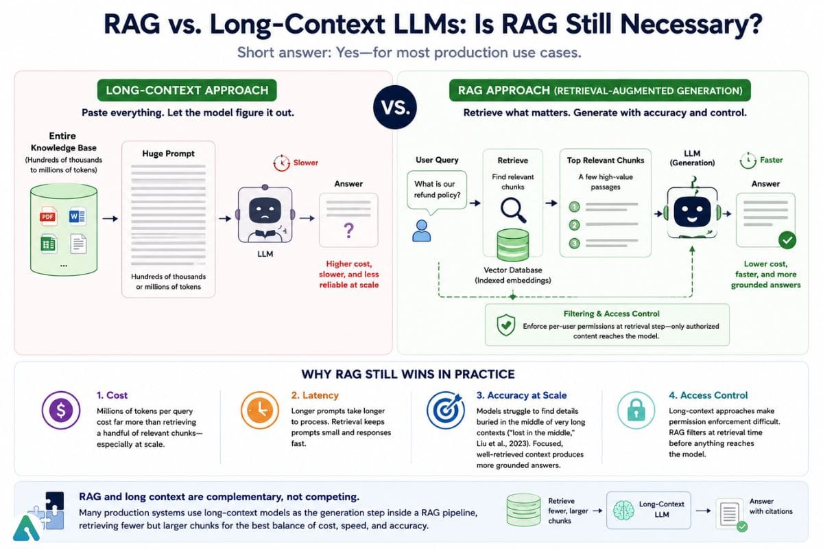
As context windows have grown into the hundreds of thousands or millions of tokens, why not just paste the entire knowledge base into the prompt? In practice, RAG still wins on most production use cases:
Cost — sending millions of tokens per query is far more expensive than retrieving a handful of relevant chunks, especially at scale.
Latency — longer prompts take longer to process; retrieval keeps prompts small and responses fast.
Accuracy at scale — models tend to lose track of details buried in the middle of very long contexts (“lost in the middle,” Liu et al., 2023), whereas focused, well-retrieved context produces more grounded answers.
Access control — long-context approaches make it harder to enforce per-user document permissions; RAG can filter at the retrieval step before anything reaches the model.
Long context windows complement RAG rather than replace it — many production systems now use a long-context model as the generation step inside a RAG pipeline, retrieving fewer but larger chunks.
Limitations of RAG Pipelines
Multi-hop reasoning — questions requiring facts connected across several unrelated documents can be difficult for standard vector retrieval; a major reason Graph RAG and Agentic RAG exist.
Ambiguous or vague queries — if the question doesn’t map clearly to specific content, retrieval quality drops.
Silent retrieval failures — if the wrong chunks are retrieved, the LLM still generates a confident-sounding answer from bad context, which can be harder to catch than an outright hallucination.
Added infrastructure and maintenance cost — a system to build, monitor, and keep in sync, not a one-time setup.
Not a fix for reasoning errors — RAG improves factual grounding, not underlying reasoning ability.
What a RAG Pipeline Costs to Build and Run
Cost center
What drives it
Embedding generation
Priced per token/document; scales with re-indexing frequency
Vector database hosting
Managed options (Pinecone, Weaviate Cloud) charge by storage and query volume; self-hosted (Chroma, Qdrant, Milvus) shifts cost to infrastructure
LLM generation calls
Priced per token at query time; lower than long-context since only retrieved chunks are sent
A small internal tool indexing a few hundred documents can run on free/low-cost open-source vector database tiers. An enterprise deployment indexing millions of documents needs more, and reranking plus hybrid search on every query is closer to a standard production service than a lightweight add-on.
Simple cost model:
Indexing cost ≈ (number of chunks) × (embedding cost per chunk) × (re-indexing frequency)
Query cost    ≈ (queries per month) × (retrieval + reranking + LLM generation cost per query)
Indexing cost mostly depends on how often the knowledge base changes; query cost mostly depends on traffic volume. High-traffic consumer-facing systems invest more heavily in caching and reranking efficiency than low-traffic internal tools.
Prompt caching as a cost lever: popular retrieved chunks and system instructions get reused across queries. Prompt caching lets the LLM provider skip reprocessing that repeated content — typically an 80–90% discount on cached input tokens, plus faster time-to-first-token. This is a big reason token-heavy techniques like Contextual Retrieval stay financially practical at production scale.
A Simple Example
A mid-sized company has a 300-page internal HR policy document. Pasting the whole document into every query would be slow and expensive, and important details would get lost. Instead, the pipeline chunks it into roughly 400–600 sections, embeds them, and stores them in a vector database. When an employee asks “how many weeks of parental leave do I get,” the pipeline retrieves the two or three chunks discussing parental leave, and the LLM answers using just that context — with a citation back to the specific policy section — instead of a generic or guessed answer.
Because RAG pipelines often connect to private company data, permissions matter as much as accuracy. Metadata filtering combined with role-based access control (RBAC) — ideally enforced through pre-filtering — ensures a user only retrieves chunks from documents they’re actually allowed to see, which is critical in HR, legal, healthcare, or financial deployments.
Common RAG-specific security risks:
Prompt injection through retrieved documents — a malicious or compromised document contains hidden instructions attempting to override the system prompt when retrieved
Indirect prompt injection — the injected instruction arrives via a trusted source (email, web page, shared document) rather than the user’s own query
Cross-tenant data leakage — a misconfigured filter lets one customer’s query retrieve another customer’s private data
Excessive permissions — a service account or retriever with broader access than necessary widens the blast radius if compromised
Malicious or poisoned documents — an attacker inserts misleading content so it gets retrieved and treated as ground truth
Sensitive information exposure — retrieved chunks surface PII, credentials, or confidential data that should never have reached the prompt
Citation or source manipulation — content crafted to be cited as authoritative, exploiting user trust in RAG citations
RAG vs. AI Agents, and What Is Agentic RAG?
Traditional RAG runs a single, fixed retrieval step per query: embed the question, retrieve chunks, generate an answer.
An AI agent plans a sequence of actions, calls tools/APIs, and decides what to do next based on intermediate results — retrieval is just one of many possible actions.
Agentic RAG applies agent-style decision-making to retrieval specifically: the system can search multiple sources, run a follow-up search based on initial results, call an external API for data outside the vector database, or flag that a claim needs verification.
Agentic RAG is worth the complexity when: the question requires multi-hop reasoning across sources, the right source isn’t known in advance, some needed information lives outside the vector database, or accuracy is high-stakes enough to justify explicit verification.
Traditional RAG is the better fit when: the knowledge base is well-scoped, most questions map to a single retrieval pass, and added latency/cost of multi-step reasoning isn’t worth it.
How to Evaluate a RAG Pipeline
Retrieval and generation can each fail independently, so evaluation splits into two categories.
Retrieval metrics — did the pipeline find the right information?
Precision — of the chunks retrieved, how many were actually relevant?
Recall — of all relevant chunks that existed, how many did retrieval find?
Context precision/recall — the same measured specifically on context reaching the LLM after reranking
MRR (Mean Reciprocal Rank) — how high up the ranked list did the first relevant result land?
NDCG — rewards relevant results ranking higher, not just appearing somewhere on the list
Generation metrics — did the model use that information correctly?
Faithfulness — does the answer match the retrieved context without unsupported claims?
Answer relevance — does the response address what was actually asked?
Correctness — is the final answer factually accurate?
Citation accuracy — do cited sources actually support the specific claims attributed to them?
Latency deserves its own tracking as a system-level metric: query embedding, index search, reranking, and generation each eat a slice of total response time. Optimizing usually means finding which single stage dominates, rather than tuning all four evenly — measure directly against your own pipeline rather than assuming a general figure.
Evaluation frameworks:RAGAS, DeepEval, TruLens, and LangSmith are common choices over manual spot-checks. A useful mental model is the RAG Triad: Context Relevance (did retrieval find the right chunks?), Groundedness (does the context support the answer?), and Answer Relevance (does the answer address the question?).
Types of RAG Pipelines
Naive RAG — the basic retrieve-then-generate flow
Advanced RAG — adds reranking, query rewriting, and hybrid search
Graph RAG — retrieves from a knowledge graph instead of (or alongside) a vector database, useful when entity relationships matter (e.g., “which suppliers are connected to products manufactured in this region?”)
Agentic RAG — an agent decides dynamically which sources to search, in what order, and whether results need verification
Multimodal RAG — retrieves and reasons over text, images, tables, audio, or video
Self-RAG — the model outputs reflection tokens judging its own process: whether retrieval is needed, whether retrieved chunks are relevant, whether the answer is supported
Corrective RAG (CRAG) — a lightweight evaluator scores retrieved chunk quality before generation; low confidence triggers a fallback to external web search or a clarifying question
RAG Architecture Decision Tree
A quick way to pick a starting pattern based on what you’re actually building:
Simple internal FAQs, well-scoped knowledge base → Naive RAG
Answers depend on relationships between entities (suppliers, org charts, dependency graphs) → Graph RAG
Multi-step, multi-source questions where the right source isn’t known ahead of time → Agentic RAG
This isn’t a strict decision procedure — most production systems start with Naive or Advanced RAG and only add Graph or Agentic patterns once a specific limitation (multi-hop questions, unknown source routing) actually shows up in evaluation.
Cloud platforms — AWS (Bedrock, Kendra, SageMaker), Azure, Google Cloud
RAG Across Industries
Healthcare — surfacing answers from medical research and hospital knowledge bases
Education — letting students query textbooks and course materials directly
Legal — searching contracts and case documents for relevant clauses
E-commerce — answering product and customer-support questions accurately
Banking — retrieving internal policy and financial documentation
HR — answering employee questions about benefits and policy
Customer support — grounding chatbot answers in product manuals and FAQs
Conclusion
A RAG pipeline solves the two biggest limitations of standalone LLMs: stale knowledge and hallucination-prone answers. By retrieving relevant, current information before generating a response, it lets AI systems stay accurate, current, and traceable back to real sources — without the cost and delay of retraining a model every time something changes. If you’re starting out, begin with the basic pipeline, get evaluation in place early, and layer in reranking and hybrid search once you see where retrieval quality actually breaks down.
Disclaimer: This article is for informational and educational purposes only. RAG technology, AI models, and best practices evolve quickly, so specific tools and recommendations may change. Always test RAG systems in your own environment and apply appropriate security, privacy, and human oversight, especially when working with sensitive or business-critical data.
Tags:
Sebastian Vale
Sebastian Vale reviews the latest AI tools and tech innovations, breaking down complex concepts into clear, actionable insights. He also creates step-by-step guides, helping readers make smarter decisions and stay ahead in a fast-moving digital world.